Revising and editing some old posts(2010). As always, your comments are desired.
Let's pick a simple example and use it to transform and illustrate the work as we go, y = x^2 -5x - 6 .
The first easy thing is to abandon the y=Ax2 + Bx + C approach for the vertex form. The equation y=A(x-h)2 + k can be easily transformed into the vector form (x,y) = (h, k) + (t, At2 ) , but in thinking about extending the power of this model, I thought it better to write it as (x,y) = (h, k) + t(1,0) + At2 (0,1). At first this seems an insignificant change, even making it more complex, but whether this was done immediately, or somewhat later in the sequence, as I will try to show, there are advantages to having a pair of perpendicular unit vectors in the equation.
So in vertex form, we write our sample equation as \( y=(x-5/2)^2 - 1/4 \). The vector form is (x,y) = (5/2, -1/4) + (t,t^2) , with the extended form of (x,y) = (5/2, -1/4) +t(1,0) + t^2 (0,1) . ( I think students could make this translation quickly because it is similar to the elements of the basic quadratic equation form.)
The first obvious advantage is that transformations no longer have the confusing sign reversal in translation of a graph (“to move the vertex three to the right, you replace x with x-3”). To move the graph to the right, simply increase the value of h, the x-coordinate of the vertex.
What about the other things we normally do with quadratics? To solve y=0 or find roots we still want to find where y=0, so k+At2 = 0. If we confine ourselves to dealing only with quadratics that are functions of y in terms of x, then the entire section on quadratic equations and completing the square (except for their historical interest and geometric interest) is now resolved by the simple two steps of setting
 and then finding the values of x from x=h+/-t. For reasons that will be more obvious later, however, we still need to develop the traditional approaches to solving quadratics.
Notice how separating the x and y components of the vector make this easy. With our example case, we set \( t= \sqrt \frac{1/4}{1} = 1/2.
evaluating (x,y) = (5/2, -1/4) +1/2(1,0) + (1/2)^2 (0,1) = (5/2, -1/4) +(1/2,0) + (0,1/4)= (3,0). By symmetry we know the other zero is (2,0).
It would seem that a little more time and emphasis on converting the general y=Ax2 + Bx + C form to the vertex form would be essential, but the savings in other areas and the increase in understanding would seem obvious.
To find values of y as a function of x, the simple expedient of solving for t makes the mysterious reversal of sign for transformations in the old form seem obvious. We change x=h+t into t=x-h; and then evaluate y=k+A(x-h)2 just as we always have. Perhaps the exception to “as we always did” is that a student now understands a little better what s/he is doing.
So what can we do we couldn’t do before? Suppose we now want to write the equation of a parabola that is not expressible as y=f(x). As a simple example, I will show how to easily write the equation of a parabola with a standard curvature (A=1) with a vertex at (2, -3) an the axis of symmetry rotated 45o.
It is for this problem that I think the three part, (x,y) = (h, k) + t(1,0) + At^2(0,1), model is needed. All we need to do is replace the two unit vectors in the x and y directions with the appropriate unit vectors. Since the axis is rotated 45o, we need the old x-axis to go in the (1,1) direction. The unit vector in that direction is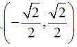 and the perpendicular to that would be
 . We simply fill in the appropriate values for the vertex and the equation is
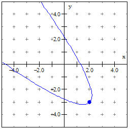
 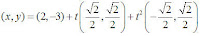 . The graph, using the parametric form in Winplot, looks like this:
To find a point of specific interest, say the x-intercepts, we can solve for t as before. Setting y = 0 we have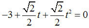 we have a typical quadratic to solve for the two values of t,
 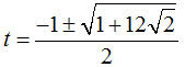 we get approximate values of –2.619 and 1.169. Then to find x we evaluate for these values of t with approximate results of x = 1.29 and x = -4.702. Solving quadratics in the traditional form will not go away.
With very little extra effort on the student’s part the student can extend this to drawing a quadratic embedded along any line in the plane, at any point. I will try to develop that in the next section of these vector blogs.
evaluating (x,y) = (5/2, -1/4) +1/2(1,0) + (1/2)^2 (0,1) = (5/2, -1/4) +(1/2,0) + (0,1/4)= (3,0). By symmetry we know the other zero is (2,0).
It would seem that a little more time and emphasis on converting the general y=Ax2 + Bx + C form to the vertex form would be essential, but the savings in other areas and the increase in understanding would seem obvious.
To find values of y as a function of x, the simple expedient of solving for t makes the mysterious reversal of sign for transformations in the old form seem obvious. We change x=h+t into t=x-h; and then evaluate y=k+A(x-h)2 just as we always have. Perhaps the exception to “as we always did” is that a student now understands a little better what s/he is doing.
So what can we do we couldn’t do before? Suppose we now want to write the equation of a parabola that is not expressible as y=f(x). As a simple example, I will show how to easily write the equation of a parabola with a standard curvature (A=1) with a vertex at (2, -3) an the axis of symmetry rotated 45o.
It is for this problem that I think the three part, (x,y) = (h, k) + t(1,0) + At^2(0,1), model is needed. All we need to do is replace the two unit vectors in the x and y directions with the appropriate unit vectors. Since the axis is rotated 45o, we need the old x-axis to go in the (1,1) direction. The unit vector in that direction is
 and the perpendicular to that would be
 . We simply fill in the appropriate values for the vertex and the equation is
  . The graph, using the parametric form in Winplot, looks like this:
To find a point of specific interest, say the x-intercepts, we can solve for t as before. Setting y = 0 we have
 we have a typical quadratic to solve for the two values of t,
  we get approximate values of –2.619 and 1.169. Then to find x we evaluate for these values of t with approximate results of x = 1.29 and x = -4.702. Solving quadratics in the traditional form will not go away.
 With very little extra effort on the student’s part the student can extend this to drawing a quadratic embedded along any line in the plane, at any point. I will try to develop that in the next section of these vector blogs.
No comments:
Post a Comment